Multiple Variable Linear Regression
Problem statement #
We will use the motivating example of housing price prediction. The training dataset contains four features (size, bedrooms, floors and, age) shown in the table below.
| Size (sqft) | Number of Bedrooms | Number of floors | Age of home (years) | Price (1,000s dollars) |
|---|---|---|---|---|
| 2104 | 5 | 1 | 45 | 460 |
| 1416 | 3 | 2 | 40 | 232 |
| 852 | 2 | 1 | 35 | 178 |
Let's build a linear regression model using these values so you can then predict the price for other houses. For example, a house with 1200 sqft, 3 bedrooms, 1 floor, 40 years old.
Matrix \(X\) containing our example #
Each row of datasets represent one example, with \(n\) number of features and \(m\) training examples, now \(\mathbf{x}\) is an input matrix with dimensions \((m, n)\) where \(m\) is row and $n$ is column.
$$\mathbf{X} = \begin{pmatrix} x^{(0)}_0 & x^{(0)}_1 & \cdots & x^{(0)}_{n-1} \\ x^{(1)}_0 & x^{(1)}_1 & \cdots & x^{(1)}_{n-1} \\ \vdots & \vdots & \vdots & \vdots \\ x^{(m-1)}_0 & x^{(m-1)}_1 & \cdots & x^{(m-1)}_{n-1} \end{pmatrix} $$
Notations
- \(\mathbf{x}^{(i)}\) is vector containing example i. \(\mathbf{x}^{(i)} = (x^{(i)}_0, x^{(i)}_1, \cdots,x^{(i)}_{n-1})\)
- \(x^{(i)}_j\) is element \(j\) in example \(i\). The superscript in parenthesis indicates the example number while the subscript represents an element.
Parameter vector \(\mathbf{w}_{j}\) , \(b\) #
-
\(\mathbf{w}\) is a vector with \(n\) elements.
- Each element contains the parameter associated with one feature.
- in our dataset, n is 4.
- notionally, we draw this as a column vector
$$\mathbf{w} = \begin{pmatrix} w_0 \\ w_1 \\ \vdots\\ w_{n-1} \end{pmatrix} $$
- \(b\) is a scalar parameter.
Load datasets #
As shown in a problem statement, our dataset contains five features (size, bedrooms, floors and, age, price of the house), \(n = 5\) and ahundred examples, \(m = 100\).
In this case our dataset will have the size of \((m , n) = (100 , 5)\)
$$\mathbf{data} = \begin{pmatrix} x^{(0)}_{0} & x^{(0)}_{1} & x^{(0)}_{2} & \cdots & y^{(0)}_{n-1} \\ x^{(1)}_{0} & x^{(1)}_{1} & x^{(1)}_{2} & \cdots & y^{(1)}_{n-1} \\ \vdots & \vdots & \vdots & \vdots & \vdots\\ x^{(m-1)}_{0} & x^{(m-1)}_{1} & x^{(m-1)}_{2} & \cdots & y^{(m-1)}_{n-1} \end{pmatrix} = \begin{pmatrix} x^{(0)}_{0} & x^{(0)}_{1} & x^{(0)}_{2} & x^{(0)}_{3} & y^{(0)}_{4} \\ x^{(1)}_{0} & x^{(1)}_{1} & x^{(1)}_{2} & x^{(1)}_{3} & y^{(1)}_{4} \\ \vdots & \vdots & \vdots & \vdots & \vdots\\ x^{(99)}_{0} & x^{(99)}_{1} & x^{(99)}_{2} & x^{(99)}_{3} & y^{(99)}_{4} \end{pmatrix} $$
$$data \in \mathbb{R}_{m \times n} = \mathbb{R}_{100 \times 5}$$
Load input datasets, \(\mathbf{x}^{(i)}_{j}\) #
Input datasets will comprise of five features (size, bedrooms, floors and, age), \(n = 4\) and hundred exaples, \(m = 100\).
$$\mathbf{X} = \begin{pmatrix} x^{(0)}_{0} & x^{(0)}_{1} & \cdots & x^{(0)}_{n-1} \\ x^{(1)}_{0} & x^{(1)}_{1} & \cdots & x^{(1)}_{n-1} \\ \vdots & \vdots & \vdots & \vdots \\ x^{(m-1)}_{0} & x^{(m-1)}_{1} & \cdots & x^{(m-1)}_{n-1} \end{pmatrix} = \begin{pmatrix} x^{(0)}_{0} & x^{(0)}_{1} & x^{(0)}_{2} & x^{(0)}_{3} \\ x^{(1)}_{0} & x^{(1)}_{1} & x^{(1)}_{2} & x^{(1)}_{3} \\ \vdots & \vdots & \vdots & \vdots \\ x^{(99)}_{0} & x^{(99)}_{1} & x^{(99)}_{2} & x^{(99)}_{3} \end{pmatrix} $$
$$\mathbf{X} \in \mathbb{R}_{m \times n} = \mathbb{R}_{100 \times 4}$$
Load output datasets, \(\mathbf{y}^{(i)}_{j}\) #
Input datasets will comprise of only one features (price), $n = 1$ and hundred exaples, $m = 100$.
$$\mathbf{Y} = \begin{pmatrix} y^{(0)}_{0} \\ y^{(1)}_{0} \\ \vdots \\ y^{(m-1)}_{0} \end{pmatrix} = \begin{pmatrix} y^{(0)}_{0} \\ y^{(1)}_{0} \\ \vdots \\ y^{(99)}_{0} \end{pmatrix} $$
$$Y \in \mathbb{R}_{m \times n} = \mathbb{R}_{100 \times 1}$$
Initialize parameters \(\mathbf{w}_{j}\) , b#
-
\(\mathbf{w}_{j}\) is a vector with $n = 4$ elements.
- Each element contains the parameter associated with one feature.
$$\mathbf{w} = \begin{pmatrix} w_{0} \\ w_{1} \\ \vdots\\ w_{n-1} \end{pmatrix} = \begin{pmatrix} w_{0} \\ w_{1} \\ w_{2}\\ w_{3} \end{pmatrix} $$
$$\mathbf{w} \in \mathbb{R}_{n \times 1} = \mathbb{R}_{4 \times 1}$$
- \(b\) is a scalar parameter.
Model Prediction With Multiple Variables #
The model's prediction with multiple variables is given by the linear model:
$$ f_{\mathbf{w},b}(\mathbf{x}^{(i)}) = w_0x_0 + w_1x_1 +... + w_{n-1}x_{n-1} + b \tag{1}$$
or in vector Notations
$$ f_{\mathbf{w},b}(\mathbf{x}) = \mathbf{w} \cdot \mathbf{X} + \mathbf{b} \tag{2} $$
$$f_{\mathbf{w},b}(\mathbf{x}) \in \mathbb{R}_{m \times 1} = \mathbf{w} \in \mathbb{R}_{n \times 1} \cdot \mathbf{X} \in \mathbb{R}_{m \times n} + \mathbf{b} \in \mathbb{R}_{1}$$
$$f_{\mathbf{w},b}(\mathbf{x})_{m \times 1} = \mathbf{w}_{n \times 1} \cdot \mathbf{X}_{m \times n} + \mathbf{b}_{1}$$
$$f_{\mathbf{w},b}(\mathbf{x}^{(i)}) \in \mathbb{R}_{m \times 1}$$
$$f_{\mathbf{w},b}(\mathbf{x}) = \begin{pmatrix} f_{\mathbf{w},b}(\mathbf{x})^{(0)}_{0} \\ f_{\mathbf{w},b}(\mathbf{x})^{(1)}_{0} \\ \vdots \\ f_{\mathbf{w},b}(\mathbf{x})^{(m-1)}_{0} \end{pmatrix} = \begin{pmatrix} f_{\mathbf{w},b}(\mathbf{x})^{(0)}_{0} \\ f_{\mathbf{w},b}(\mathbf{x})^{(1)}_{0} \\ \vdots \\ f_{\mathbf{w},b}(\mathbf{x})^{(99)}_{0} \end{pmatrix} $$
where \(\cdot\) is a vector `dot product`
To demonstrate the dot product, we will implement prediction using (1) and (2).
double *predict(float **x, double w[][1], double b){

  /*
  single predict using linear regression

  Args:
    x (ndarray): Shape (m, n) example with multiple features
    w (ndarray): Shape (n, 1) model parameters
    b (scalar):  model parameter

  Returns:
    p (scalar):  prediction

  */

  double p;
  double *f_wb=(double *)malloc(m*sizeof(double));
  if (f_wb==NULL)
  {
    perror("Error allocating memory");
    free(f_wb);
  }


  for (int i = 0; i < m; i++)
  {
    for (int j = 0; j < 1; j++)
    {
      p=0;
      for (int k = 0; k < n; k++)
      {
          p += (double)x[i][k]*w[k][j];
      }
      p += b;
      f_wb[i]=p;

    }
  }

  return f_wb;
}
Compute Cost With Multiple Variables #
The equation for the cost function with multiple variables \(J(\mathbf{w},b)\) is:
$$J(\mathbf{w},b) = \frac{1}{2m} \sum\limits_{i = 0}^{m-1} (f_{\mathbf{w},b}(\mathbf{x}^{(i)}) - y^{(i)})^2 \tag{3}$$ where: $$ f_{\mathbf{w},b}(\mathbf{x}^{(i)}) = \mathbf{w} \cdot \mathbf{X} + b \tag{4} $$
$$f_{\mathbf{w},b}(\mathbf{x}) \in \mathbb{R}_{m \times 1}$$
In contrast to previous labs, \(\mathbf{w}\) and \(\mathbf{x}^{(i)}\) are vectors rather than scalars supporting multiple features.
double compute_cost(float **x, float y[m], double w[][1], double b){

  /*
    compute cost
  Args:
    X (ndarray (m,n)): Data, m examples with n features
    y (ndarray (m,1)) : target values
    w (ndarray (n,1)) : model parameters
    b (scalar)       : model parameter

  Returns:
    cost (scalar): cost

  */

  double cost=0;
  double p;

  for (int i = 0; i < m; i++)
  {
    for (int j = 0; j < 1; j++)
    {
      p=0;
      for (int k = 0; k < n; k++)
      {
        p += (double)x[i][k]*w[k][j];
      }
      p +=b;
    }
    cost += pow((p - (double) y[i]), 2);
  }
  cost /= (2*m);

  return cost;
}
Gradient Descent With Multiple Variables#
Gradient descent for multiple variables:
$$\begin{align*} \text{repeat}&\text{ until convergence:} \; \lbrace \newline\; & w_j = w_j - \alpha \frac{\partial J(\mathbf{w},b)}{\partial w_j} \tag{5} \; & \text{for j = 0..n-1}\newline &b\ \ = b - \alpha \frac{\partial J(\mathbf{w},b)}{\partial b} \newline \rbrace \end{align*}$$
where, n is the number of features, parameters $w_j$, $b$, are updated simultaneously and where
$$ \begin{align} \frac{\partial J(\mathbf{w},b)}{\partial w_j} &= \frac{1}{m} \sum\limits_{i = 0}^{m-1} (f_{\mathbf{w},b}(\mathbf{x}^{(i)}) - y^{(i)})x_{j}^{(i)} \tag{6} \\ \frac{\partial J(\mathbf{w},b)}{\partial b} &= \frac{1}{m} \sum\limits_{i = 0}^{m-1} (f_{\mathbf{w},b}(\mathbf{x}^{(i)}) - y^{(i)}) \tag{7} \end{align} $$
- m is the number of training examples in the data set
- \(f_{\mathbf{w},b}(\mathbf{x}^{(i)})\) is the model's prediction, while \(y^{(i)}\) is the target value
Note
-
$$\frac{\partial J(\mathbf{w},b)}{\partial w_j} \in \mathbb{R}_{1 \times n} = \mathbb{R}_{1 \times 4}$$
$$\frac{\partial J(\mathbf{w},b)}{\partial w_j} = \begin{pmatrix} \frac{\partial J(\mathbf{w},b)}{\partial w_0} , \frac{\partial J(\mathbf{w},b)}{\partial w_1} , \cdots , \frac{\partial J(\mathbf{w},b)}{\partial w_{n-1}} \end{pmatrix} = \begin{pmatrix} \frac{\partial J(\mathbf{w},b)}{\partial w_0} , \frac{\partial J(\mathbf{w},b)}{\partial w_1} , \frac{\partial J(\mathbf{w},b)}{\partial w_2} , \frac{\partial J(\mathbf{w},b)}{\partial w_3} \end{pmatrix} $$
- $$\frac{\partial J(\mathbf{w},b)}{\partial b} \in \mathbb{R}_{1}$$
double *compute_gradient(float **x, float y[m], double w[][1], double b){
  /*

  Computes the gradient for linear regression
  Args:
    X (ndarray (m,n)): Data, m examples with n features
    y (ndarray (m,1)) : target values
    w (ndarray (n,1)) : model parameters
    b (scalar)       : model parameter

  Returns:
    dj_dw (ndarray (n,1)): The gradient of the cost w.r.t. the parameters w.
    dj_db (scalar):       The gradient of the cost w.r.t. the parameter b.

    grads (ndarray ((n+1), 1)): dj_dw and dj_db.
  */

  double *grads=(double *)malloc((n + 1)*sizeof(double));
  if (grads ==NULL)
  {
      perror("Error in allocating memory");
      free(grads);
  }

  double *f_wb=(double *)malloc(m*sizeof(double));
  if (f_wb ==NULL)
  {
      perror("Error in allocating memory");
      free(f_wb);
  }

  double p;
  double dj_dw;
  double dj_db=0;

  for (int i = 0; i < m; i++)
  {
    for (int j = 0; j < 1; j++)
    {
      p=0;
      for (int k = 0; k < n; k++)
      {
        p += x[i][k]*w[k][j];
      }
      p += b;
      f_wb[i]=p;
    }

    dj_db += f_wb[i] - y[i];
  }
  dj_db /= m;


  for (int i = 0; i < n; i++)
  {
    dj_dw=0;
    for (int j = 0; j < m; j++)
    {
      dj_dw += (f_wb[j] - y[j])*x[j][i];
    }
    dj_dw /= m;

    grads[i]=dj_dw;
  }

  grads[n]=dj_db;

  free(f_wb);

  return grads;
}
Evaluating our model by compute R-squared#
R-squared is the proportion of the variance in the dependent variable that is explained by the independent variables in a regression model. It ranges from 0 to 1, where 0 means no relationship and 1 means a perfect fit
R-squared(coefficient of Determination) tells us How well our model is performing or how well our model's predictions match the real results. A higher R-squared means our model is doing a better job predicting.
$$ R^2 = 1 - \frac{Residual\ Sum\ of\ Squares\ (\mathbf{ss}_{res})}{Total\ Sum\ of\ Squares\ (\mathbf{ss}_{total})} $$
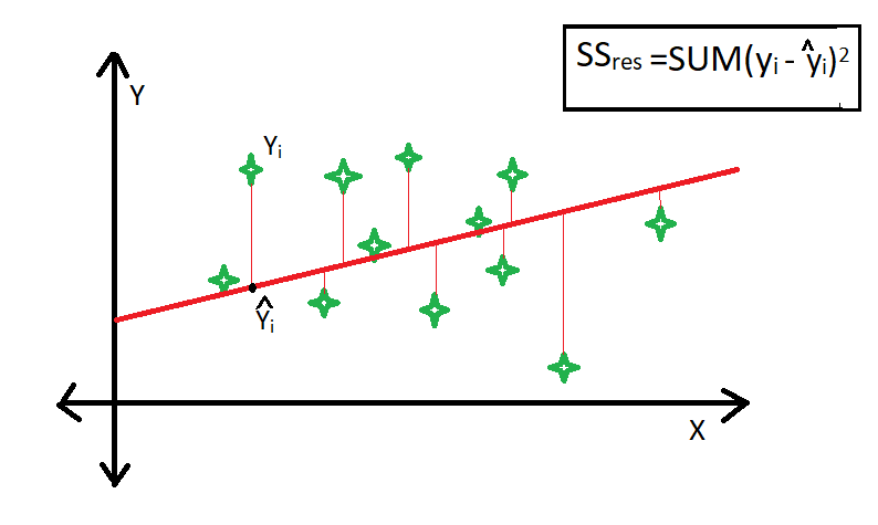
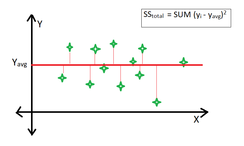
$$ R^2 = 1 - \frac{\mathbf{ss}_{res}}{\mathbf{ss}_{total}}\\ $$
$$ R^2 = 1 - \frac{\sum\limits_{i=0}^{(m-1)}(f_{w,b}(x^{(i)}) - y^{i})^2}{\sum\limits_{i=0}^{(m-1)}(y_{mean}^{(i)} - y^{(i)})^2} $$
double r_squared(float **x, float y[m], double w[][1], double b){

  /*

  Computes the gradient for linear regression
  Args:
    X (ndarray (m,n)): Data, m examples with n features
    y (ndarray (m,1)) : target values
    w (ndarray (n,1)) : model parameters
    b (scalar)       : model parameter

  Returns:
    r_square (scalar): r square score.
    r_square = (1 - rss/tss)
    rss : measure of sum diff btn actual(y) value and predicted(f_wb) value.(y - f_wb)
    tss : measure of total variance in actual(y) value. (y - f_mean)

  */

  double r_square;
  double f_wb;
  double y_mean;
  double y_sum;
  double rss;
  double tss;

  for (int i = 0; i < m; i++)
  {
    for (int j = 0; j < 1; j++)
    {
      f_wb=0;
      for (int k = 0; k < n; k++)
      {
        f_wb += x[i][k]*w[k][j];
      }
      f_wb +=b;
    }

    rss += pow((y[i] - f_wb), 2);
    y_sum += y[i];

  }
  y_mean = y_sum/m;

  for (int i = 0; i < m; i++)
  {
    tss += pow((y[i] - y_mean), 2);
  }

  r_square = 1 - (rss/tss);


  return r_square;
}