Univariate Linear Regression
Problem statement #
Suppose you are the CEO of a restaurant franchise and are considering different cities for opening a new outlet.
- You would like to expand your business to cities that may give your restaurant higher profits.
- The chain already has restaurants in various cities and you have data for profits and populations from the cities.
- You also have data on cities that are candidates for a new restaurant.
- For these cities, you have the city population.
Can you use the data to help you identify which cities may potentially give your business higher profits?
Note:
- 'X' is the population of a city
- 'y' is the profit of a restaurant in that city. A negative value for profit indicates a loss.
- Both 'X' and 'y' are arrays.
| Population of a city (x 10,000) as \(x\) | Profit of a restaurent (x $10,000) as \( f_{w,b}(x^{(i)}) \)or \(x\) |
|---|---|
| 6.1101 | 17.592 |
| 5.5277 | 9.1302 |
| 8.5186 | 13.662 |
| 7.0032 | 11.854 |
| 5.8598 | 6.8233 |
Number of training example (size (1000 sqft) as x) \(m\)
In this case \(m = 5\)
Model Function #
The model function for linear regression (which is a function that maps from \(x\) to \(y\) is represented as
$$f_{w,b}(x^{(i)}) = w*x^{(i)} + b \tag{1}$$
float *compute_model_output(float x[], float w, float b, int m){

  /*
  Computes the prediction of a linear model
  Args:
  X[m] (ndarray (m,1)): Data, m examples
  w,b (scalar)     : model parameters
  m (scalar)       : number of examples, X
  Returns
  Y[m] (ndarray (m,1)): target values
  */

  float *f_x = (float *)malloc(m * sizeof(float));

  for(int i = 0; i < m; i++){
    f_x[i] = x[i] * w + b;
  }
  return f_x;
}
Compute Cost #
Cost is the measure of how well our model will predict the target output well, in this case target output is Profit of a restaurent.
Gradient descent involve repeated steps to adjust the values of w and b to get smaller and smaller Cost, \(J(w,b)\).
The equation for Cost with one variable
$$J(w,b) = \frac{1}{2m} \sum\limits_{i = 0}^{m-1} (f_{w,b}(x^{(i)}) - y^{(i)})^2 \tag{2}$$where
$$f_{w,b}(x^{(i)}) = w*x^{(i)} + b \tag{1}$$- \(f_{w,b}(x^{(i)}) \)is our prediction for example $i$ using parameters \(w,b\).
- \((f_{w,b}(x^{(i)}) -y^{(i)})^2\) is the squared difference between the target value and the prediction.
- These differences are summed over all the $m$ examples and divided by 2*m to produce the cost, \(J(w,b)\).
Note,
- Summation ranges are typically from 1 to m, while code will be from 0 to m-1.
float compute_cost(float x[], float y[], float w, float b, int m){

  /*
  Computes the cost function for linear regression.

  Args:
  X (ndarray (m,1)): Data, m examples
  Y (ndarray (m,1)): target values
  w,b (scalar)     : model parameters
  m (scalar)       : number of examples, X

  Returns
    total_cost (float): The cost of using w,b as the parameters for linear regression
          to fit the data points in X and Y
  */

  float J_wb = 0;
  float f_x;

  for (int i = 0; i < m; i++)
  {
    f_x = x[i] * w + b;
    J_wb += pow((f_x - y[i]), 2);
  }
  J_wb /= (2 * m);

  return J_wb;
}
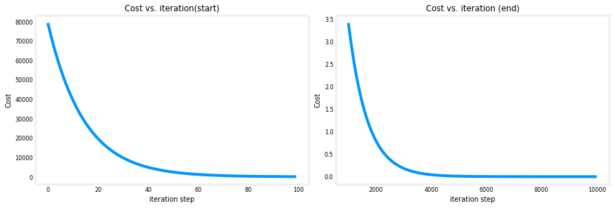
Cost versus iterations of gradient descent #
A plot of cost versus iterations is a useful measure of progress in gradient descent. Cost should always decrease in successful runs. The change in cost is so rapid initially, it is useful to plot the initial decent on a different scale than the final descent. In the plots below, note the scale of cost on the axes and the iteration step.
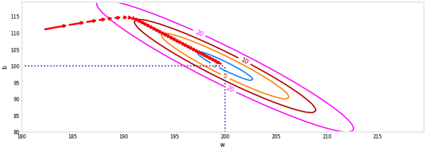
Plot of cost J(w,b) vs w,b with path of gradient descent #
Plot shows the $cost(w,b)$ over a range of $w$ and $b$. Cost levels are represented by the rings. Overlayed, using red arrows, is the path of gradient descent. Here are some things to note:
- The path makes steady (monotonic) progress toward its goal.
- initial steps are much larger than the steps near the goal.
Convex Cost surface #
The fact that the cost function squares the loss, \( \sum_{i = 0}^{m-1} (f_{w,b}(x^{(i)}) - y^{(i)})^2\) ensures that the 'error surface' is convex like a soup bowl. It will always have a minimum that can be reached by following the gradient in all dimensions.
Gradient Descent #
In linear regression, we utilize input training data to fit the parameters \(w\),\(b\) by minimizing a measure of the error between our predictions \(f_{w,b}(x^{(i)})\) and the actual data \(y^{(i)}\). The measure is called the $cost$, \(J(w,b)\). In training you measure the cost over all of our training samples \(x^{(i)},y^{(i)}\)
$$\begin{align*} \text{repeat}&\text{ until convergence:} \; \lbrace \newline \; w &= w - \alpha \frac{\partial J(w,b)}{\partial w} \tag{3} \; \newline b &= b - \alpha \frac{\partial J(w,b)}{\partial b} \newline \rbrace \end{align*}$$where, parameters \(w\), \(b\) are updated simultaneously.
The gradient is defined as:
$$ \begin{align} \frac{\partial J(w,b)}{\partial w} &= \frac{1}{m} \sum\limits_{i = 0}^{m-1} (f_{w,b}(x^{(i)}) - y^{(i)})*x^{(i)} \tag{4}\\ \frac{\partial J(w,b)}{\partial b} &= \frac{1}{m} \sum\limits_{i = 0}^{m-1} (f_{w,b}(x^{(i)}) - y^{(i)}) \tag{5}\\ \end{align} $$Here *simultaniously* means that you calculate the partial derivatives for all the parameters before updating any of the parameters.
float *compute_gradients(float x[], float y[], float w, float b, int m){

  /*
  Computes the gradients w,b for linear regression
  Args:
  x (ndarray (m,1)): Data, m examples
  y (ndarray (m,1)): target values
  w,b (scalar)    : model parameters
  m (scalar)       : number of examples, X
  Returns
  dj_dw (scalar): The gradient of the cost w.r.t. the parameters w
  dj_db (scalar): The gradient of the cost w.r.t. the parameters b
  grads (ndarray (2,1)): gradients [dj_dw, dj_db]
  */

  float f_x;
  float dj_dw = 0;
  float dj_db = 0;
  float *grads = (float *)malloc(2 * sizeof(float));

  for (int i = 0; i < m; i++)
  {
    f_x = x[i] * w + b;
    dj_dw += (f_x - y[i]) * x[i];
    dj_db += (f_x - y[i]);
  }
  dj_dw /= m;
  dj_db /= m;

  grads[0] = dj_dw;   //index 0: dj_dw
  grads[1] = dj_db;   //index 1: dj_db

  return grads;
}
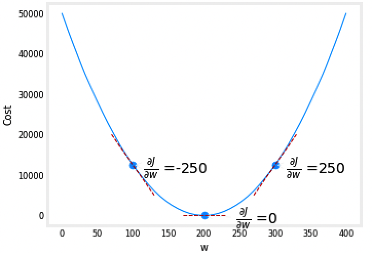
Cost vs w, with gradients, b set to 100 #
The plot shows \(\frac{\partial J(w,b)}{\partial w}\) or the slope of the cost curve relative to \(w\) at three points. The derivative is negative. Due to the 'bowl shape', the derivatives will always lead gradient descent toward the bottom where the gradient is zero.
Evaluating our model #
To evaluate the estimation model, we use coefficient of determination which is given by the following formula:
$$ R^2 = 1 - \frac{Residual\ Square\ Sum}{Total\ Square\ Sum} $$ $$ R^2 = 1 - \frac{\sum\limits_{i=0}^{(m-1)}(f_{w,b}(x^{(i)}) - y^{i})^2}{\sum\limits_{i=0}^{(m-1)}(f_{w,b}(x^{(i)}) - f_{w,b}(x^{(i)})_{mean})^2} $$float *compute_weight_bias(float w, float b, float dj_dw, float dj_db, float alpha){ /* Performs gradient descent to fit w,b. Updates w,b by taking gradient steps with learning rate alpha Args: w,b (scalar): initial values of model parameters alpha (float): Learning rate dj_dw (scalar): The gradient of the cost w.r.t. the parameters w dj_db (scalar): The gradient of the cost w.r.t. the parameters b Returns: w (scalar): Updated value of parameter after running gradient descent b (scalar): Updated value of parameter after running gradient descent p_hist (ndarray (2,1)): History of parameters [w,b] */ float *p_hist = (float *)malloc(2 * sizeof(float)); w = w - (alpha * dj_dw); b = b - (alpha * dj_db); p_hist[0] = w; //weight p_hist[1] = b; //bias return p_hist; }
Learning parameters using batch gradient descent#
You will now find the optimal parameters of a linear regression model by using batch gradient descent. Recall batch refers to running all the examples in one iteration.
- You don't need to implement anything for this part. Simply run the cells below.
- A good way to verify that gradient descent is working correctly is to look at the value of \(J(w,b)\) and check that it is decreasing with each step.
- Assuming you have implemented the gradient and computed the cost correctly and you have an appropriate value for the learning rate alpha, \(J(w,b)\) should never increase and should converge to a steady value by the end of the algorithm.
Expected Output#
Optimal w, b found by gradient descent
| w | b |
|---|---|
| |-3.216610 | |-3.216610 |
We will now use our final parameters w, b to find our prediction for single example.
recall:
$$ f_{w,b}(x^{(i)}) = w * x^{i} + b $$Let's predict what profit will be for the ares of 35,000 and 70,000 people
- The model takes in population of a city in 10,000s as input.
- Therefore, 35,000 people can be translated into an input to the model as input[] = {3.5}
- Similarly, 70,000 people can be translated into an input to the model as input[] = {7.5}
The main function#
#include <stdio.h>
#include <stdlib.h>
#include <math.h>

//Initializing functions
float *compute_model_output(float x[], float w, float b, int m);
float compute_cost(float x[], float y[], float w, float b, int m);
float *compute_gradients(float x[], float y[], float w, float b, int m);
float *compute_weight_bias(float w, float b, float dj_dw, float dj_db, float alpha);
float evaluate_model(float x[], float y[], float w, float b, int m);

int main(){

  //initialize w and b
  float w_in = 0;
  float b_in = 0;

  //initialize input, x
  float x[]={6.1101, 5.5277, 8.5186, 7.0032, 5.8598,
            8.3829, 7.4764, 8.5781, 6.4862, 5.0546,
            5.7107, 14.164, 5.734, 8.4084, 5.6407,
            5.3794, 6.3654, 5.1301,6.4296, 7.0708, 6.1891};
  float y[]={17.592, 9.1302, 13.662, 11.854, 6.8233,
            11.886, 4.3483, 12, 6.5987, 3.8166, 3.2522,
            15.505, 3.1551, 7.2258, 0.71618, 3.5129,
            5.3048, 0.56077, 3.6518, 5.3893, 3.1386};

  //number of example, m
  int m = sizeof(x) / sizeof(x[0]);
  float alpha = 1e-2;
  int num_iters = 10000;

  float w = 0;
  float b = 0;
  float J_wb = 0;
  float dj_dw = 0;
  float dj_db = 0;

  for (int i = 0; i <= num_iters; i++)
  {
    // Save cost J at each iteration
    J_wb = compute_cost(x, y, w, b, m);

    // Calculate the gradient and update the parameters using gradient_function
    float *grads = compute_gradients(x, y, w, b, m);

    dj_dw = grads[0];
    dj_db = grads[1];

    // Update Parameters using equation (3) above
    float *p_hist = compute_weight_bias(w, b, dj_dw, dj_db, alpha);

    //R square
    float R_square = evaluate_model(x, y, w, b, m);

    w = p_hist[0];
    b = p_hist[1];

    // Print cost every at intervals 10 times or as many iterations if < 10
    if (ceil(i % 1000) == 0)
    {
      printf("Iteration: %5d\tCost: %10f\t R_Score: %10f\t dj_dw: %10f\t dj_db:%10f\t w: %10f\tb:%8f\n", i, J_wb, R_square, dj_dw, dj_db, w, b);
    }
  }

  //Predicting the Profit of restaurant, with a given Population, popul for 1 example, eg=1
  int eg = 2;
  float popul[] = {3.5, 7.5};

  float weight = w;
  float bias = b;
  float *pred = compute_model_output(popul, weight, bias, eg);
  for (int i = 0; i < eg; i++)
  {
    printf("\nFor population: %f,\t we predict the profit of:$ %f\n", popul[i] * 10000, pred[i] * 10000);
  }

  return 0;
}